This assignment will introduce you to OpenStreetMap feature tracing and tagging. We’ll also dig into a few open data formats and Mapbox Studio. The steps we’ll take to contribute to OpenStreetMap effectively and collaboratively are as follows:
- Sign up as a contributor to OpenStreetMap
- make an account
- go through the iD Editor Walkthrough
- practice tracing a building in State College
- Organize group mapping effort by assigning areas to specific contributors
- identify your assigned area
- select your area from a larger GeoJSON file
- convert your assigned area data from GeoJSON to a GPX file
- Edit OpenStreetMap within your assigned area
- display your assigned area as a GPX file in the iD Editor
- begin tracing buildings within your area
- tag buildings appropriately and square building polygons
- regularly save edits
- Creating before and after maps with Mapbox Studio
- create a free Mapbox starter account
- open our custom style in Mapbox Studio
- add and style vector tile source of our assigned areas
- export after-tracing image of your area
- adjust style sheet to show old building data
- export before-tracing image of your area at same dimensions
1. Become an OpenStreetMap Contributor
The first thing we’ll do is get acquainted to OpenStreetMap (OSM). Go to https://www.openstreetmap.org/user/new and make a new account. After you’ve created an account, zoom to State College on the main map. Zoom in far enough and you’ll be able to click “Edit” at the top of the page.
This will bring you to the iD Editor. The first thing you’ll see a a welcome box with an option to start a walkthrough of the editor’s functionality. Do this now.
Once you have completed the walkthrough, go to State College and try tracing a single building. Great. We’ll do a lot more of this later.
2. Tracing Assignments
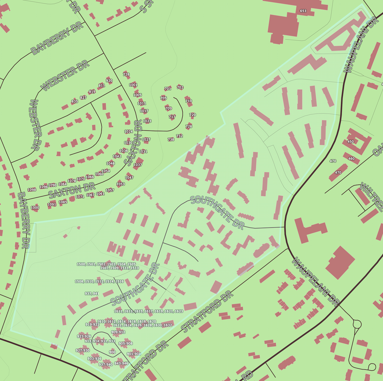
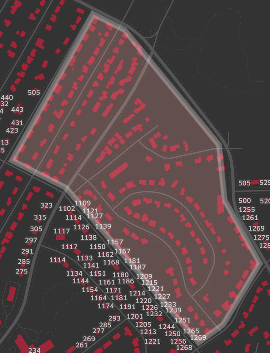
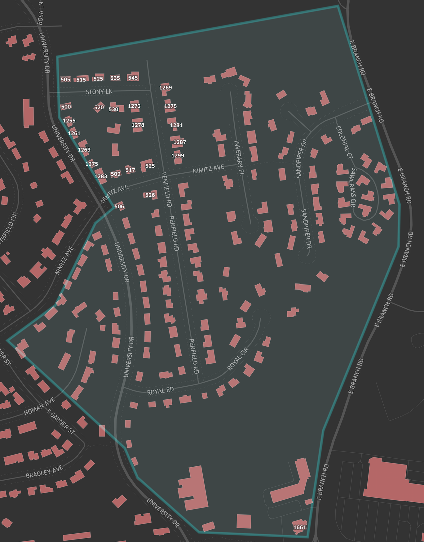
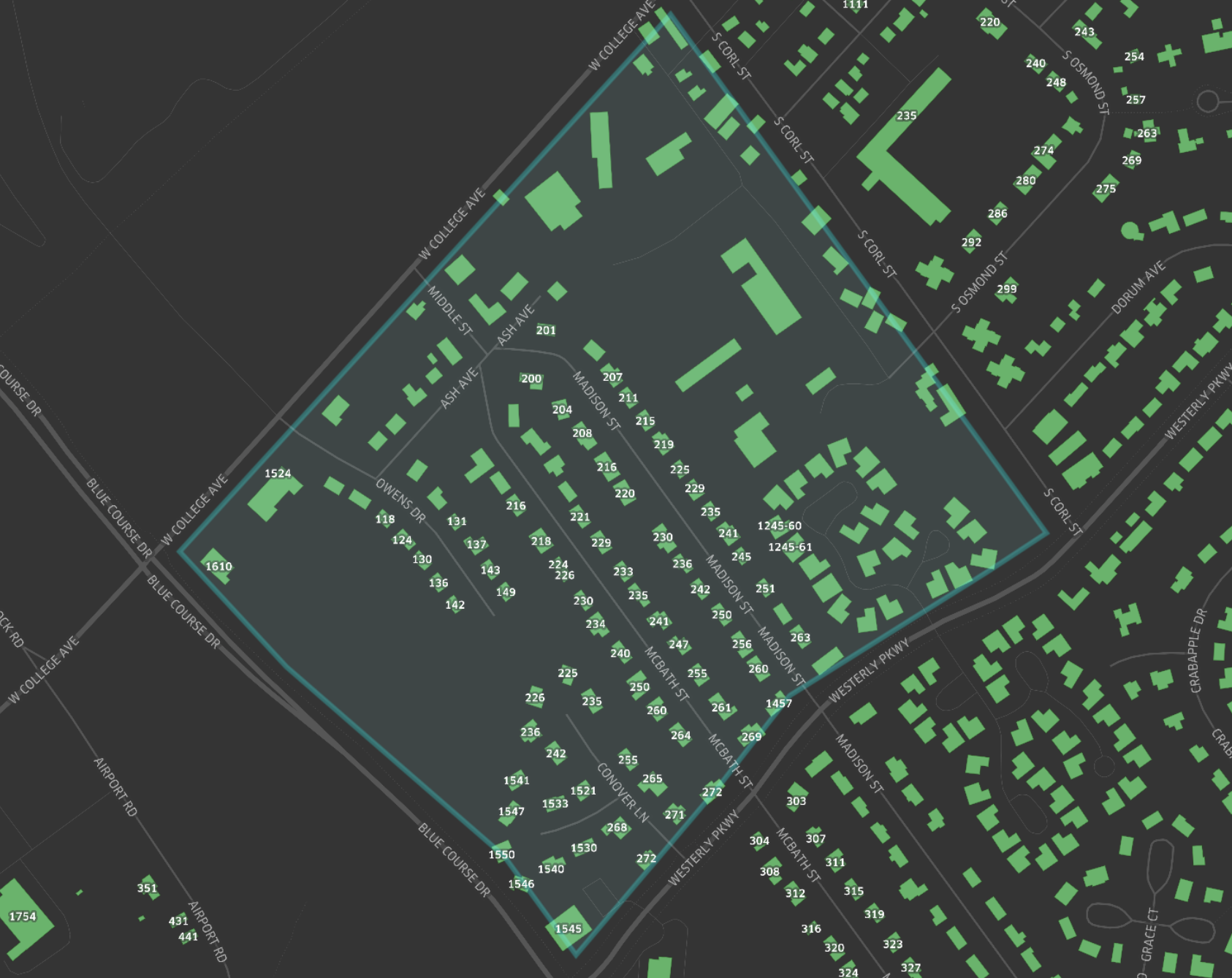
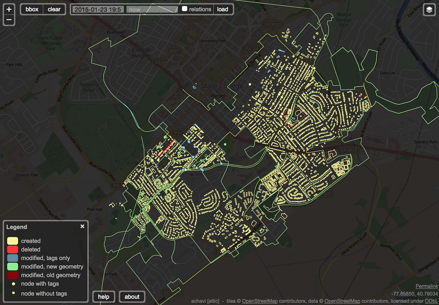
In the map below you can see State College divided into indivual sections by pink polygons. The dark grey shapes on the map show the #building layer from Mapbox Streets, a global vector tile source built and regularly updated from the OSM database. Any changes to OSM will be reflected on this map within minutes. As of January 24, 2015, many areas of the OSM database in State College could benefit from someone going through and tracing building outlines. We have assigned each section to a specific contributor. You will be using the OSM iD Editor to add building content in your assigned area. Explore the map by clicking on the pink shapes to see who was assigned to each section.
The map above renders the assigned sections by referencing a GeoJSON file. Think of a GeoJSON file as similar to a Shapefile in that it contains vector geographic data, but it’s a single text file that is human readable, instead of several files with information about geometry in the .shp file, related attributes in another file, and projection information in yet another. We use GeoJSON on the web because the text within the file is directly readable by JavaScript as data. You’ll want to have a solid understanding of this data format for the next part of the exercise. Read more about GeoJSON here.
As you know, OpenStreetMap is a collaborative database that lots of people can contribute to at any time. This also means sometimes people are unknowingly editing the same part of the map at the same time, which causes issues and ends up wasting everyone’s time. That’s why we have gone through all this trouble of dividing our mapping project–tracing buildings in State College–into different sections. You’ll be able to display the boundary of your assigned section in the OSM iD Editor as you’re editing so that you don’t step on the toes of anyone else working on the map (like the other people in this class) and they will stay clear of your section. To do that, we’ll have to take a closer look at that GeoJSON file, pull out the data relevant to you, and convert it to a data format supported by the iD Editor called a GPX file.
2a. Referencing Your Assignment in the iD Editor
To display your tracing assignment for reference in the iD Editor, we’ll need to extract your specific polygon feature from the GeoJSON file and create a GPX file. Why does it need to be a GPX file? This particular type of file has a long history with OSM and, consequently, all of the modern OSM editing tools, like the iD Editor, provide great functionality for this data format. A GPX file is what GPS receivers generate when you mark waypoints or create tracks while walking around in the field. They were especially useful in the early days of OSM when the primary method of adding roads and other features was not through tracing satellite imagery, but uploading, tracing, and editting data collected by contributors with GPS receivers. This is still a useful method today for collecting geographic data about things like trails, which often can’t be seen from space, or in places where high resolution imagery isn’t available.
We’ll be using the GPX files for the less conventional purpose of designating assigned areas for a coordinated mapping effort, although if you ever contribute to the Humanitarian OpenStreetMap Team’s collaborative mapping efforts–and you should–you’ll see their tasking manager also uses boundaries in GPX format to split a larger effort into smaller pieces.
So let’s make the GPX file you need and start mapping.
2b. Select Your Assignment from the GeoJSON
A GeoJSON file is just a text file. You can open it, copy and paste all the text it into another place, and it will still be GeoJSON. You can find the GeoJSON for the tracing assignments here.
This is the GeoJSON, and at first it probably looks like a long and confusing list of brackets, numbers, and punctuation. Let’s start with the first three lines and the last two.
{
  "type": "FeatureCollection",
  "features": [
...
  ]
}
These are the lines that set up everything else. They create what is known as an object in JavaScript. The object is a list of properties and values between the two curly braces on the first and last lines {}. One of those properties is type–in this case the value of the type property of the object is a collection of geographic features, or a FeatureCollection and the second property is features. Inside the features you’ll find another list of objects–a feature collection–contained within the two square brackets [].
{
  "type": "FeatureCollection",
  "features": [
    {
      "type": "Feature",
      "properties": {
        "contributor": "Aaron Dennis"
      },
      "geometry": {
        "type": "Polygon",
        "coordinates": [
        ...
        ]
      }
    }
  ]
}
Within the square brackets [] of the features property we see another curly brace { followed by the familiar type property. This time, the value of the type property is just Feature, not FeatureCollection. That’s because we’re now looking the GeoJSON data for a single polygon representing an individual tracing assignment. The three properties of this Feature object are type, properties, and geometry. To make an analogy to Shapefiles, properties contains all of the feature’s attribute information, like the .dbf file, and geometry contains information identifying what type of feature it is and a listing of all the coordinates for the vertices of the feature, like the .shp file.
To select your tracing assignment boundary’s Polygon Feature from within all of the features, you’ll need to create a GeoJSON with list of "features": [...] that includes only your Feature. The tool at http://geojson.io will set you up with an empty GeoJSON FeatureCollection you can copy and paste your Feature into, or you can copy and paste all the GeoJSON text I have provided into the text pane at http://geojson.io and edit it down to just your assigned feature.
2c. Convert Your GeoJSON to a GPX File
Now that you have your assigned area in GeoJSON format, it’s time to make a quick conversion to GPX. Why didn’t we just make a GPX file in the first place? Because GPX files don’t play as well with web mapping APIs like Leaflet, aren’t as readable, and you’re much less likely to use them in general. Plus, GPX files can’t actually draw polygons, just the edges of the polygon.
I’ve built an interface at http://aaronpdennis.github.io/geojson-to-gpx/ to help us convert the data. Paste your GeoJSON into the top box, click the button, and then copy and paste the code in the bottom box into a blank text document on your computer (use a basic text editor like Notepad on Windows or TextEdit on Mac OS X). Save that file with the extension .gpx.
3. Editing OpenStreetMap with the iD Editor
You’re now almost ready to start contributing to OSM. Go to OpenStreetMap.org, log in to your account, zoom to State College, and click Edit. This will bring you into the iD Editor. You will see an option on the screen to start a walkthrough of the editor’s functionality or begin editing immediately. Choose the walkthrough for your first time.
After the walkthrough, click begin editing. The first thing we’ll do is drag and drop the GPX file you saved on the computer into the iD Editor. If your GeoJSON to GPX conversion process went without any mistakes, you’ll see your assigned area rendered on the map. Now, you can start editing.
Your job is to trace all visible buildings inside your assigned area and tag them appropriately. We will talk about how to properly trace and tag OSM features in class.
4. Creating before and after maps in Mapbox Studio
Once you have thoroughly and accurately traced all buildings within your assigned area and you’ve added field-gathered address numbers for at least twenty of those buildings, you’ll be ready to create the following final deliverables for this project:
- A 300ppi PNG image exported from Mapbox Studio at zoom level 17 showing buildings and house numbers data from your area before tracing.
- A 300ppi PNG image exported from Mapbox Studio at zoom level 17 showing buildings and house numbers data from your area after tracing.
4a. Sign up for a Mapbox account
To use Mapbox Studio, you’ll need an account. Mapbox provides free access to all of its mapping and development tools with its basic “Starter” account.
4b. Getting started with Mapbox Studio
Mapbox Studio is a software application designed for making tiled web maps. It’s the new version of TileMill and there’s two really important things that it can do. The first is taking geographic data–like Shapefiles and GeoJSON–and slicing it up into square vector map tiles, which you can upload to Mapbox’s online hosting services. Vector tiles</a> are useful because they’re lightweight. This format lets us do crazy things like rendering the entire world, offline, from a USB stick. The second really important thing you can do with Mapbox Studio is reference these vector tiles and style their geometries with CartoCSS stylesheets. You can then upload these stylesheets to Mapbox and they’ll give you an API that serves up your tiles in a slippy map (like the basemap for the map at the top of this page).
We’ve installed Mapbox Studio on the computers in 208 Walker, but it’s a free software so I would also encourage you to install it on your own computer for this class or in the future. Like other free and open source software, this is something you’ll still be able to use after you graduate.
Right now, there’s an issue with the Windows version of Mapbox Studio that only lets you write to the C:\ drive. This is problematic because there’s only one place on this drive the computer lab’s security settings let you write to. So, before we start, we’ll make a folder on this drive where you can save your Mapbox Studio projects. Open Windows Explorer and navigate to C:\Users\ and then your PSU ID (xyz1234). Create a folder here called mapbox_studio. Whenever you leave this computer, copy that folder onto a flash drive as a back up. This folder will only be availble on the C:\ drive of the machine you’re using now.
I’ve set up a Mapbox Studio project for us to start out with. Download the ZIP file at this link. Then, extract the geog467-project-2.tm2 folder and copy it into your mapbox-studio folder on the C:\ drive.
Now, open the Mapbox Studio program on your computer.
You’ll be prompted to sign in. This will allow you to upload styles and sources to Mapbox. After signing in, you’ll see a variety of styles the cartographers at Mapbox have designed. Pick one that seems interesting and check it out.
Once you’ve clicked on a style, you’ll see stylesheets full of CartoCSS on the right, a map pane in the middle, and a column with buttons that pull out drawers like “settings”, “layers”, “fonts”, “docs”, and “projects” on the left. Click on “docs” and then click on the blue “Interface tour” button. Read through this.
We’re now going to open the project in the .tm2 folder that you saved to the C:\ drive. Click on the “Projects” button in the bottom left, then “Browse” to the geog467-project-2.tm2 project. Open it, and you’ll be looking at State College.
4c. Adding a custom vector source for old buildings data and assignments
Before we started this project, I downloaded the OSM data for State College and then used QGIS to extract building polygons and create points for house number labels. I then used Mapbox Studio to make this data into a vector tile source and upload it to Mapbox. I’ve made this vector tile source public, so you’re now able to reference it and style it in your Mapbox Studio styles.
In the “layers” drawer on the left, you’ll see an option to “Change source”. Clicking here brings you to a window with a list of sources you can use. Right now, the project is using mapbox.mapbox-streets-v5, but mapbox also provides global vector tile sources for terrain, with #hillshade, #contour, and #landcover, and a satellite source to add their imagery basemap.
The source I made has the ID aarondennis.f7666d1c. If you put a comma , after mapbox.mapbox-streets-v5and then paste in aarondennis.f7666d1c, you’ll add these custom vector tiles to the project. Your source reference should now be mapbox.mapbox-streets-v5,aarondennis.f7666d1c. Click apply and then save your project. The layers panel should now show a layer for #building_old, #assignments, and #housenum_label_old.
In the CartoCSS editor on the right, click on the tab labeled “buildings”. Copy and paste the code below onto line 17. This will style the #assignments layer in the custom source you just added. Save the project and you should see the assignment areas added to the map in blue.
#assignments {
  polygon-fill: #95ffff;
  polygon-opacity: 0.1;
  line-color: #00ffff;
  line-width: 5;
  line-opacity: 0.3;
  comp-op: screen;
  image-filters: agg-stack-blur(4,4);
  image-filters-inflate: true;
}
The text you see on the “style” and “buildings” tabs are style sheets that dictate what you see on the map. Writing #building { polygon-fill: red; } would show the #building layer on the map as red shapes. There’s a lot of different ways to style points, lines, polygons, raster, and text. The “Docs” drawer gives you a list of all the posibilities.
This is a cartography class and I hope you take the liberty to tweak a few things in this style I’ve provided. Make it your own, create your own flair. Just remember to keep sound cartographic principles and aesthetics in mind.
The features on the map also have fields with values (or attributes) associated to them. In the “Layers” drawer, click on the #assignments layer. This layer has a field called contributor and has the name of the person assigned to each feature as a value. You can use the syntax [field='value'] after your #layer in CartoCSS to select features and style them a certain way.
Do this for your #assignments layer so that the map only shows the area assigned by you. Your CartoCSS should look like the text below, with your name typed exactly as it appears on the GeoJSON map at the beginning of this assignment.
#assignments [contributor='Your Name'] {
  ...
}
Save your project and you should see the assignment areas updated to show only your area.
4d. Export after-tracing image of your area
The map on your screen is a reflection of the current state of the OSM database. Recall that the mapbox.mapbox-streets-v5 is built from planet wide OSM data and updated every few minutes. You can probably see buildings on this map that you were tracing in the iD Editor just earlier today. Right now, the map shows all the contributions our class has made to OSM buildings in State College. In the next steps, we will save this map as an image, and then we’ll look at what building data existed before we started tracing.
While Mapbox Studio is best known for designing web map tiles, it also has some great print functionality. In the upper right corner, above all the CartoCSS, is a hard to notice button that looks like some sort of picture icon. Clicking here brings us into Mapbox Studio’s export image functionality. This is where you will make those final deliverables we mentioned earlier. Zoom in or out to Zoom Level 17, frame the box nicely around your assigned area, and then download a 300 pixel-per-inch PNG image file to your mapbox-studio folder. This is your “after-tracing” image.
4e. Adjust style sheet to show old building data
Close out of the image exporter and go back to the building style sheet. Change #building and #housenum_label to #building_old and #housenum_label_old so that they reference the layers of before-tracing data in the custom vector tile source I provided. Save it and watch all the buildings we’ve traced disappear, leaving many neighborhoods in State College barren of building data, just as it was before we started all this.
4f. Export before-tracing image of your area at same dimensions
If you go back to the image export screen, you should be able to download another image at the same dimensions and crop bounds. This will be your “before-tracing” map. Make sure it shows exactly the same area and is also rendered at Zoom Level 17.
Congratulations!
To recap, we’ve dug into GeoJSON, converted file formats, got familiar with the iD OSM editor, contributed significantly to the OSM data in State College, learned a little bit about Mapbox Studio, and made some maps showing our progress.
Results
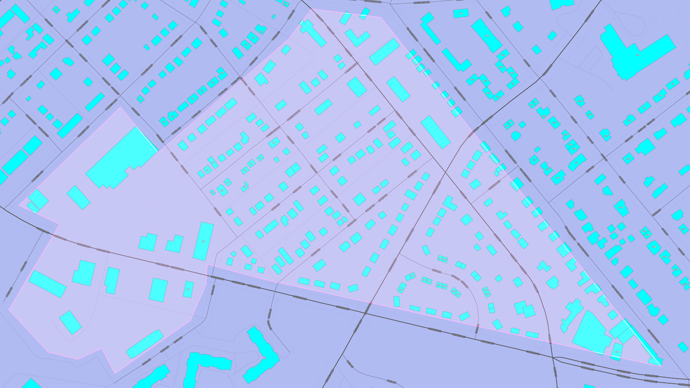
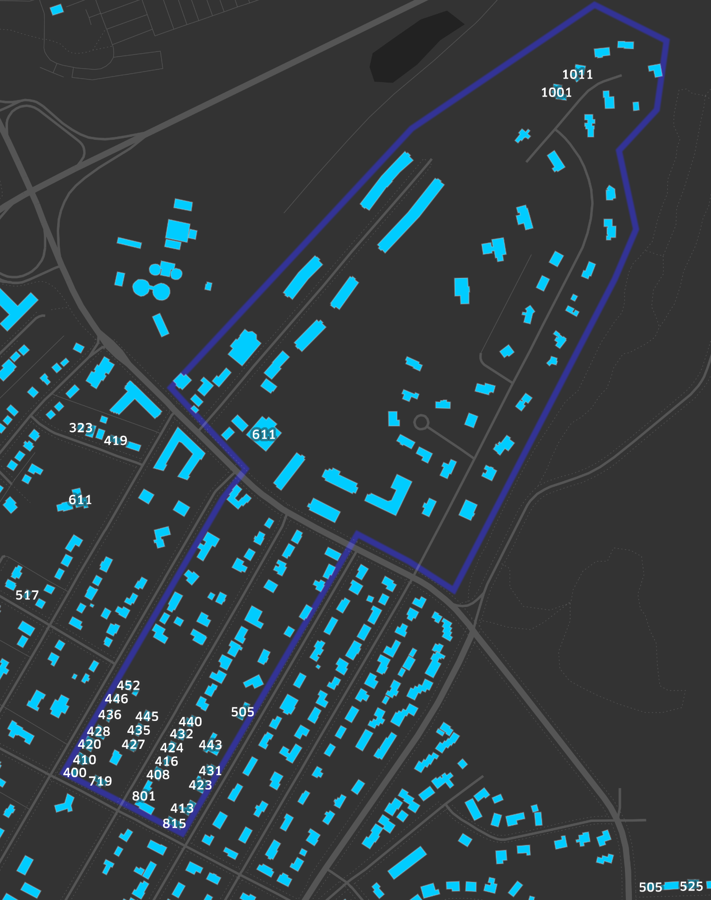
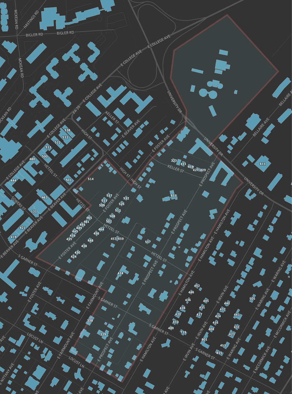
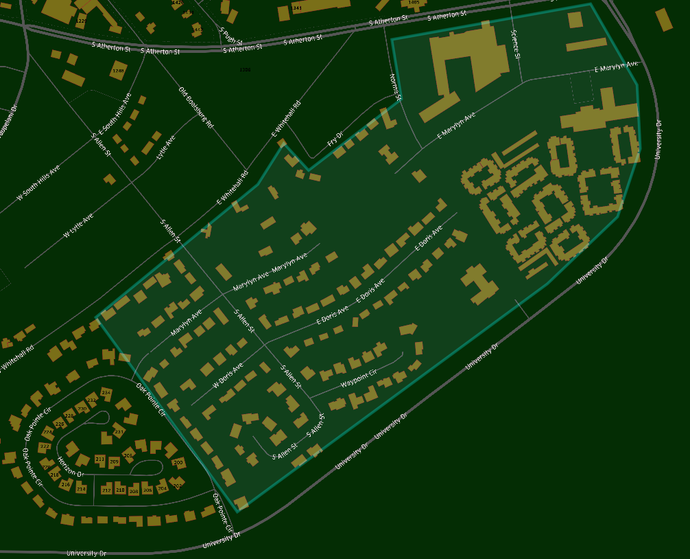
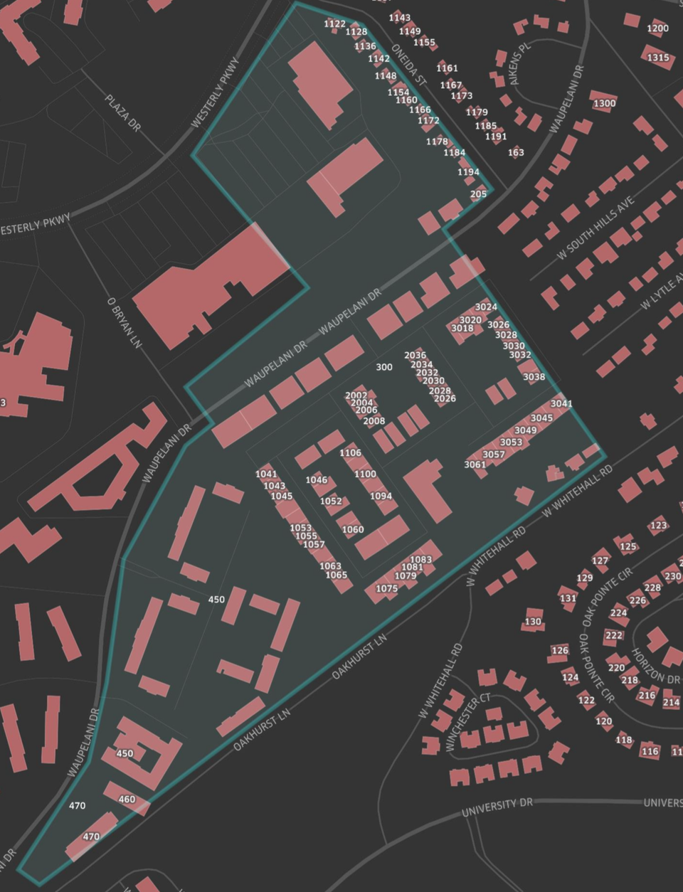
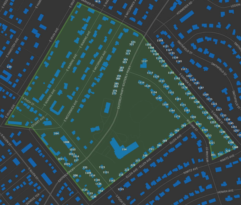
Since beginning this project, we have contributed significantly to the OSM database in State College. The figure below shows in yellow all new features created during our two week project. Of these features, approximately 25% have full attribution including address numbers.
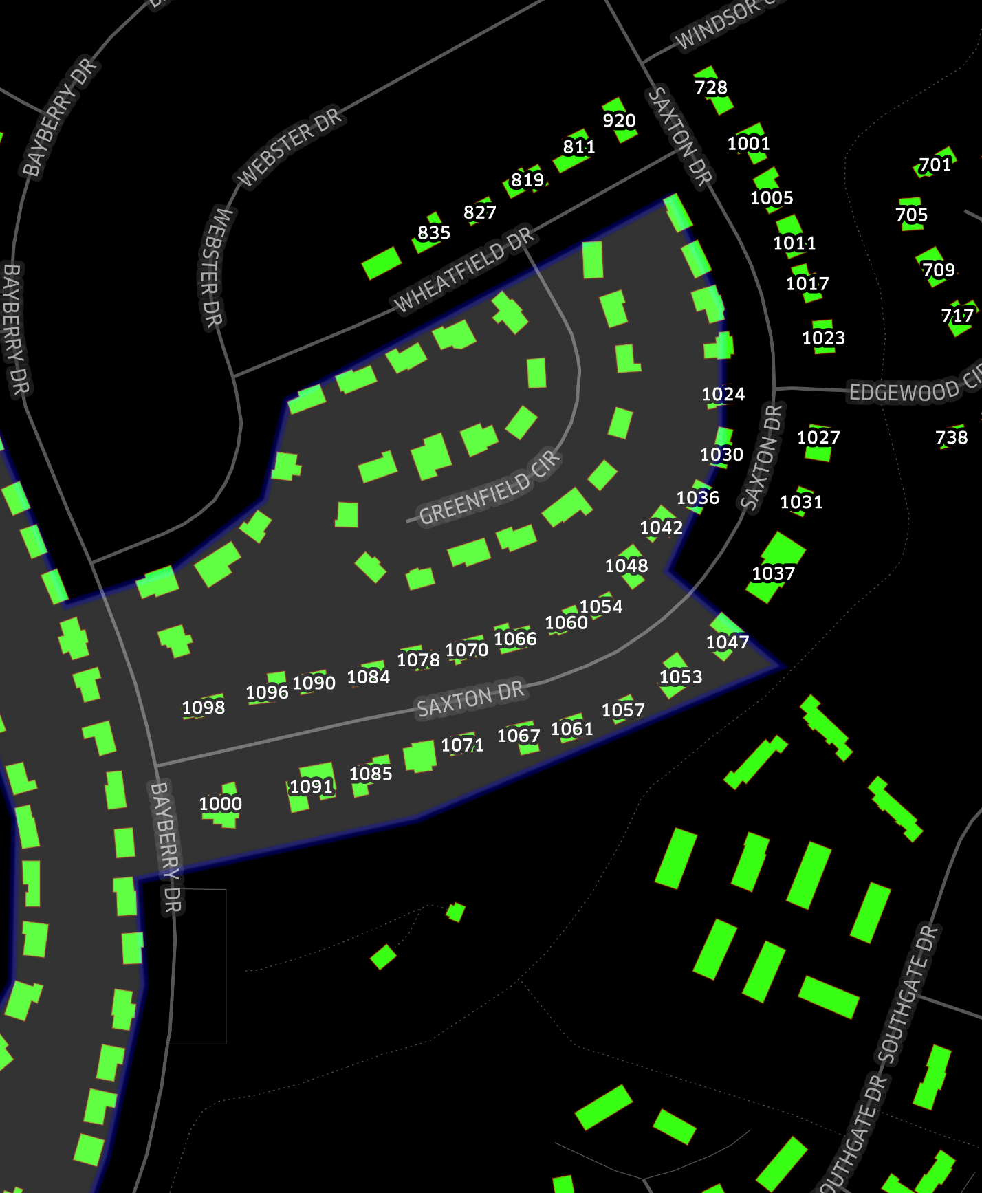
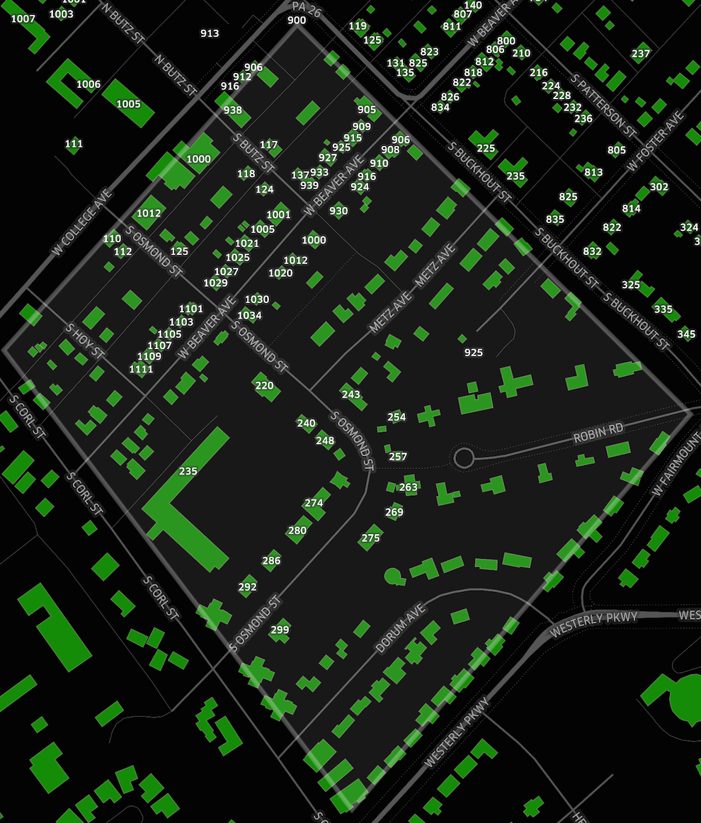
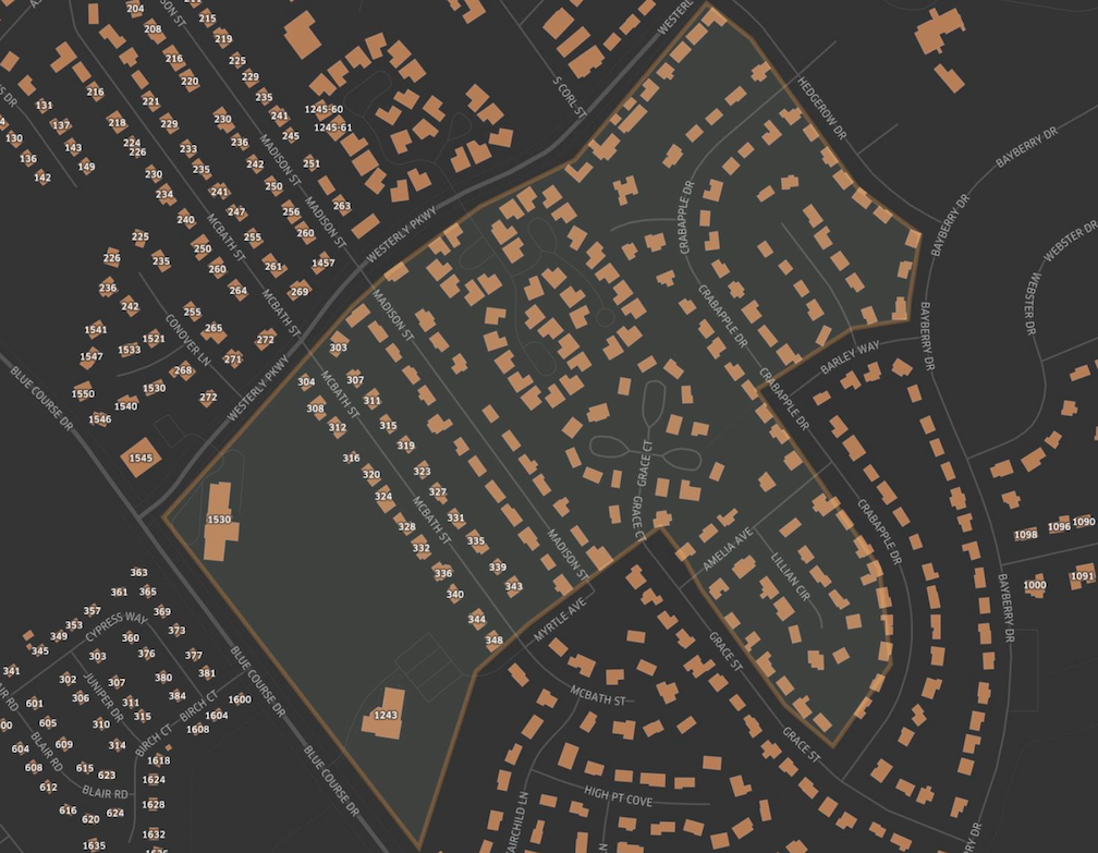
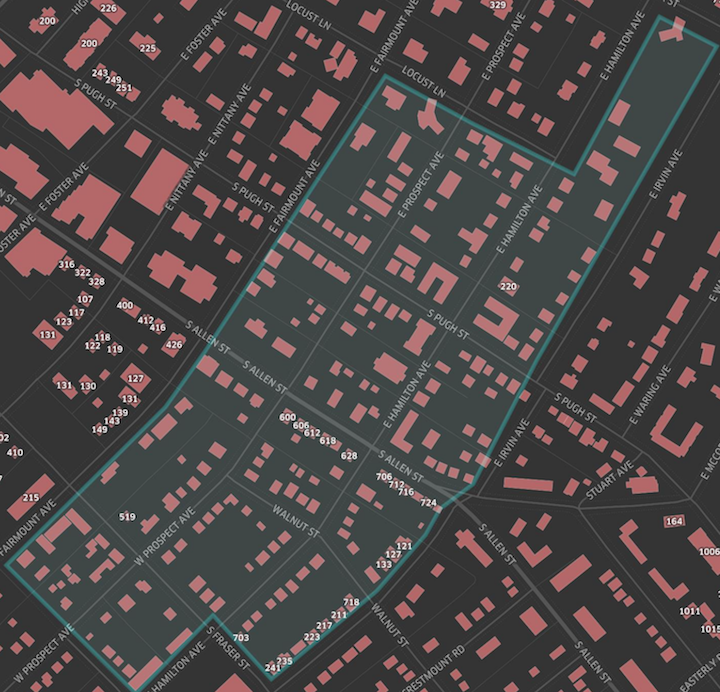
Some of the after-tracing maps that we generated in Mapbox Studio are included below.